Mini-Project #02: Making Backyards Affordable for All
Author
Apu Datta
Introduction
Housing affordability has become one of the most urgent policy challenges in the United States, particularly in high-cost metropolitan regions such as New York City, San Francisco, and Boston. Many local zoning and permitting practices have restricted new housing construction, driving up prices and limiting access for working families. In contrast, a growing movement known as YIMBY (“Yes In My Back Yard”) argues that cities can become more affordable, diverse, and dynamic by relaxing restrictive zoning rules and encouraging denser, mixed-use development. Opposing this stance are NIMBY (“Not In My Back Yard”) groups who resist additional housing in their neighborhoods.
YIMBY vs NIMBY Housing Illustration
🏙️ This project investigates where U.S. housing markets demonstrate pro-YIMBY patterns—where new housing construction is keeping pace with demand.
Mini-Project #02: “Making Backyards Affordable for All” challenges students to identify America’s most YIMBY-friendly metropolitan areas using multiple public datasets. Inspired by urban-planning analyses from Ray Delahanty (CityNerd), this project merges data from the U.S. Census Bureau’s American Community Survey (ACS) and the Bureau of Labor Statistics (BLS) to explore where rent growth, income trends, and new housing permits intersect. The analysis is performed using R and emphasizes the tidycensus, dplyr, and ggplot2 packages.
Urban Housing Skyline
🧰 Learning Objectives
Students will: - Practice data acquisition and integration with dplyr joins and key alignment across Census and BLS tables.
- Use basic visual analytics with ggplot2 to reveal affordability patterns.
- Construct interpretable indices such as Rent Burden and Housing Growth Rate to quantify affordability.
- Communicate results effectively to a non-technical policymaking audience through clear narrative and visuals.
🪜 Analytical Workflow
Data Acquisition – download and prepare ACS and BLS datasets.
Data Integration and Initial Exploration – join tables, ensure consistent CBSA identifiers, and answer exploratory questions.
Visualization – create supporting plots showing rent vs income and household size trends.
Metric Construction – compute and standardize rent-burden and housing-growth indices.
Policy Brief – summarize findings for decision-makers and identify ideal congressional sponsors.
Data Flow Diagram – ACS, BLS, and Derived Metrics
🎯 Focus of This Project
This mini-project emphasizes data alignment, descriptive analysis, and storytelling over predictive modeling. While modeling and inference will appear in later assignments, MP02 demonstrates how structured public data can provide insights into how YIMBY-style housing policies influence affordability and community growth across U.S. cities. The final policy brief will synthesize these findings into a concise and persuasive argument supporting a national pro-YIMBY initiative.
Data Acquisition
🧩 Task 1: Data Import and Preparation
In this section, I downloaded and prepared all datasets necessary for my analysis of housing affordability.
I relied primarily on two U.S. government sources — the American Community Survey (ACS) from the U.S. Census Bureau and the Quarterly Census of Employment and Wages (QCEW) from the Bureau of Labor Statistics (BLS).
Each dataset was saved in a local directory named data/mp02.
The following code includes all instructor-provided functions and automated download steps. —
1️⃣ Creating the Data Directory and Package Setup
The first step ensures that the working directory contains a folder to store all downloaded datasets and loads every required R package.
📦 Click to see the code
# --- Step 1: Create data folder if it doesn't exist ---if(!dir.exists(file.path("data", "mp02"))){dir.create(file.path("data", "mp02"), showWarnings=FALSE, recursive=TRUE)}# --- Step 2: Custom library() function to auto-install missing packages ---library <-function(pkg){ pkg <-as.character(substitute(pkg))options(repos =c(CRAN ="https://cloud.r-project.org"))if(!require(pkg, character.only=TRUE, quietly=TRUE)) install.packages(pkg)stopifnot(require(pkg, character.only=TRUE, quietly=TRUE))}# --- Step 3: Load required packages ---library(tidyverse)library(glue)library(readxl)library(tidycensus)library(stringr)library(cli)
🪄 Results:
This code first makes a new folder called data/mp02 to store all downloaded files. Then it checks that I have the needed R packages (like tidyverse, glue, readxl, etc.). If any are missing, it installs them automatically and loads them so that project runs smoothly. —
2️⃣ Downloading ACS Data (Income, Rent, Population, Households)
I used the get_acs_all_years() helper function to pull annual CBSA-level estimates for key socioeconomic indicators from 2009–2023, excluding 2020 due to COVID-19 data gaps.
🏗️ Click to see the ACS Download Code
# --- Function to Download ACS Data (Income, Rent, Population, Households) ---get_acs_all_years <-function(variable, geography ="cbsa",start_year =2009, end_year =2023) { fname <-glue("{variable}_{geography}_{start_year}_{end_year}.csv") fname <-file.path("data", "mp02", fname)if (!file.exists(fname)) { YEARS <-seq(start_year, end_year) YEARS <- YEARS[YEARS !=2020] # Drop 2020 cli::cli_alert_info("Downloading ACS {variable} for {length(YEARS)} years ({min(YEARS)}–{max(YEARS)})...") ALL_DATA <- purrr::map( YEARS,function(yy) { tidycensus::get_acs(geography, variable, year = yy, survey ="acs1") |> dplyr::mutate(year = yy) |> dplyr::select(-moe, -variable) |> dplyr::rename(!!variable := estimate) },.progress =FALSE ) |> dplyr::bind_rows() readr::write_csv(ALL_DATA, fname) cli::cli_alert_success("Saved ACS {variable} to {fname}.") } else { cli::cli_alert_success("Using cached ACS {variable} from {fname}.") } readr::read_csv(fname, show_col_types =FALSE)}
# --- Call the function for all required variables ---INCOME <-get_acs_all_years("B19013_001") |>rename(household_income = B19013_001)RENT <-get_acs_all_years("B25064_001") |>rename(monthly_rent = B25064_001)POPULATION <-get_acs_all_years("B01003_001") |>rename(population = B01003_001)HOUSEHOLDS <-get_acs_all_years("B11001_001") |>rename(households = B11001_001)
🪄 Result:
This code downloads data from the U.S. Census Bureau for every year between 2009 and 2023 (skipping 2020 because of missing data). It collects information about:
💵 Income (median household income)
🏠 Rent (average monthly rent)
👨👩👧 Population (total people living in the area)
🏘️ Households (total number of homes)
If already have the data saved in data/mp02 folder, it won’t download again, it just reuses the saved file. This saves time and avoids unnecessary downloads every time run the report.
3️⃣ Collecting Building Permit Data
Because the number of newly permitted housing units is not available in tidycensus, I imported this information manually from the U.S. Census Bureau’s construction statistics.
🏗️ Click to see the code
# --- Step 1: Define the function that downloads or loads building-permit data ---get_building_permits <-function(start_year =2009, end_year =2023){ fname <-glue("housing_units_{start_year}_{end_year}.csv") fname <-file.path("data", "mp02", fname)if(!file.exists(fname)){ cli::cli_alert_info("Downloading building permits (historical and current)...")# 2009–2018 historical text files HISTORICAL_YEARS <-seq(start_year, 2018) HISTORICAL_DATA <- purrr::map( HISTORICAL_YEARS,function(yy){ historical_url <-glue::glue("https://www.census.gov/construction/bps/txt/tb3u{yy}.txt") LINES <-readLines(historical_url)[-c(1:11)] CBSA_LINES <- stringr::str_detect(LINES, "^[[:digit:]]") CBSA <-as.integer(stringr::str_sub(LINES[CBSA_LINES], 5, 10)) PERMIT_LINES <- stringr::str_detect(stringr::str_sub(LINES, 48, 53), "[[:digit:]]") PERMITS <-as.integer(stringr::str_sub(LINES[PERMIT_LINES], 48, 53)) tibble::tibble(CBSA = CBSA, new_housing_units_permitted = PERMITS, year = yy) },.progress =TRUE ) |> dplyr::bind_rows()# 2019–2023 Excel-format files CURRENT_YEARS <-seq(2019, end_year) CURRENT_DATA <- purrr::map( CURRENT_YEARS,function(yy){ current_url <- glue::glue("https://www.census.gov/construction/bps/xls/msaannual_{yy}99.xls") temp <-tempfile()download.file(current_url, destfile = temp, mode="wb") fallback <-function(.f1, .f2){ function(...){ tryCatch(.f1(...), error=function(e) .f2(...)) } } reader <-fallback(readxl::read_xlsx, readxl::read_xls)reader(temp, skip=5) |> tidyr::drop_na() |> dplyr::select(CBSA = dplyr::any_of(c("CBSA", "CBSA Code", "CBSAcode")),Total = dplyr::any_of(c("Total", "TOTAL")) ) |> dplyr::mutate(CBSA =as.integer(CBSA),year = yy,new_housing_units_permitted =as.integer(Total) ) |> dplyr::select(CBSA, new_housing_units_permitted, year) },.progress =TRUE ) |> dplyr::bind_rows()# Combine both and save ALL_DATA <-rbind(HISTORICAL_DATA, CURRENT_DATA) readr::write_csv(ALL_DATA, fname) cli::cli_alert_success("Saved building permits to {fname}.") } else { cli::cli_alert_success("Using cached building permits from {fname}.") }read_csv(fname, show_col_types=FALSE)}# --- Step 2: Run the function and store the result ---PERMITS <-get_building_permits()
✔ Using cached building permits from data/mp02/housing_units_2009_2023.csv.
🪄 Result:
This code first defines a function that knows how to download U.S. Census building permit data for every metro area (CBSA) between 2009 and 2023. Then, it runs that function to either:
📥 Download new data (if missing), or
💾 Load the saved data (if it already exists).
4️⃣ Understanding Core-Based Statistical Areas (CBSA)
📍 Why Use the CBSA Level?
A Core-Based Statistical Area (CBSA) represents a metro or micro area built around a main urban center and its economically linked surroundings. All data sources in this project from the American Community Survey and Bureau of Labor Statistics to Census building permits are collected at the CBSA level.
This standardization ensures that housing, income, and employment data align consistently across regions, making analysis fair and comparable.
5️⃣ Downloading BLS Industry and Wage Data
The next steps use BLS sources to enrich our dataset with employment and income structure.
🏢 Click to see industry code function (get_bls_industry_codes)
library(httr2)library(rvest)# NOTE: This function downloads the NAICS hierarchy (industry titles) from bls.gov# and shapes it into a clean table with level1–level4 titles & codes.get_bls_industry_codes <-function(){ fname <-file.path("data", "mp02", "bls_industry_codes.csv")library(dplyr); library(tidyr); library(readr)if(!file.exists(fname)){ cli::cli_alert_info("Downloading BLS NAICS industry codes...")# Build request to the BLS industry titles page resp <-request("https://www.bls.gov") |>req_url_path("cew", "classifications", "industry", "industry-titles.htm") |>req_headers(`User-Agent`="Mozilla/5.0 (Windows NT 10.0; Win64; x64) AppleWebKit/537.36 (KHTML, like Gecko) Chrome/120.0.0.0 Safari/537.36",`Accept-Language`="en-US,en;q=0.9",`Accept`="text/html,application/xhtml+xml" ) |># Don't error hard on HTTP status; handle afterreq_error(is_error = \(resp) FALSE) |>req_perform()# Validate response statusresp_check_status(resp)# Parse the NAICS table in the HTML page naics_table <-resp_body_html(resp) |>html_element("#naics_titles") |>html_table() |>mutate(title =str_trim(str_remove(str_remove(`Industry Title`, Code), "NAICS"))) |>select(-`Industry Title`) |>mutate(depth =if_else(nchar(Code) <=5, nchar(Code) -1, NA)) |>filter(!is.na(depth))# Manually add ranges that appear compressed on the page naics_missing <- tibble::tribble(~Code, ~title, ~depth,"31","Manufacturing",1,"32","Manufacturing",1,"33","Manufacturing",1,"44","Retail",1,"45","Retail",1,"48","Transportation and Warehousing",1,"49","Transportation and Warehousing",1) naics_table <-bind_rows(naics_table, naics_missing)# Keep a copy of all levels to join titles across the hierarchy naics_all <- naics_table # Build a clean 4-level hierarchy table with integer codes naics_table <- naics_table |>filter(depth ==4) |>rename(level4_title = title) |>mutate(level1_code =str_sub(Code, end =2),level2_code =str_sub(Code, end =3),level3_code =str_sub(Code, end =4),level4_code = Code ) |>left_join(naics_all |>select(Code, title), by =c("level1_code"="Code")) |>rename(level1_title = title) |>left_join(naics_all |>select(Code, title), by =c("level2_code"="Code")) |>rename(level2_title = title) |>left_join(naics_all |>select(Code, title), by =c("level3_code"="Code")) |>rename(level3_title = title) |>select(level1_title, level2_title, level3_title, level4_title, level1_code, level2_code, level3_code, level4_code) |>mutate(level1_code =suppressWarnings(as.integer(level1_code)),level2_code =suppressWarnings(as.integer(level2_code)),level3_code =suppressWarnings(as.integer(level3_code)),level4_code =suppressWarnings(as.integer(level4_code)) ) readr::write_csv(naics_table, fname) cli::cli_alert_success("Saved industry codes to {fname}.") } else { cli::cli_alert_success("Using cached industry codes from {fname}.") }read_csv(fname, show_col_types=FALSE)}
🪄 Result:
This defines a function that downloads industry titles (NAICS) from BLS, builds a 4-level industry hierarchy, saves it to a CSV, and reuses that file next time.
▶ Click to see industry code download call
# Run the function once; returns a clean NAICS hierarchy tableINDUSTRY_CODES <-get_bls_industry_codes()
✔ Using cached industry codes from data/mp02/bls_industry_codes.csv.
🪄 Result:
This line runs the function above and stores the table in INDUSTRY_CODES. If the CSV already exists, it loads it; otherwise it downloads and saves it. —
💵 Click to see wage data function (get_bls_qcew_annual_averages)
# NOTE: This function downloads annual QCEW "singlefile" ZIPs for each year (except 2020),# filters to CBSA rows and ≤5-digit NAICS, computes average wage,# writes a compressed CSV once, then reuses it on later runs.get_bls_qcew_annual_averages <-function(start_year=2009, end_year=2023){ fname <-glue("bls_qcew_{start_year}_{end_year}.csv.gz") fname <-file.path("data", "mp02", fname) YEARS <-seq(start_year, end_year) YEARS <- YEARS[YEARS !=2020]if(!file.exists(fname)){ ALL_DATA <- purrr::map( YEARS, purrr::possibly(function(yy) { fname_inner <-file.path("data", "mp02", glue("{yy}_qcew_annual_singlefile.zip"))if(!file.exists(fname_inner)){request("https://www.bls.gov") |>req_url_path("cew","data","files",yy,"csv",glue("{yy}_annual_singlefile.zip")) |>req_headers(`User-Agent`="Mozilla/5.0 (Windows NT 10.0; Win64; x64) AppleWebKit/537.36 (KHTML, like Gecko) Chrome/120.0.0.0 Safari/537.36",`Accept-Language`="en-US,en;q=0.9",`Accept`="text/html,application/xhtml+xml" ) |>req_retry(max_tries=5) |>req_perform(fname_inner)if (file.info(fname_inner)$size <755e5) {warning(sQuote(fname_inner), " appears corrupted. Please delete and retry this step.") } } readr::read_csv(fname_inner, show_col_types =FALSE) |> dplyr::mutate(YEAR = yy,annual_avg_emplvl =as.numeric(annual_avg_emplvl),total_annual_wages =as.numeric(total_annual_wages) ) |> dplyr::select(area_fips, industry_code, annual_avg_emplvl, total_annual_wages, YEAR) |> dplyr::filter(nchar(industry_code) <=5, stringr::str_starts(area_fips, "C"),!stringr::str_detect(industry_code, "-") ) |> dplyr::mutate(FIPS = area_fips,INDUSTRY =as.integer(industry_code),EMPLOYMENT =as.integer(annual_avg_emplvl),TOTAL_WAGES = total_annual_wages ) |> dplyr::select(-area_fips, -industry_code, -annual_avg_emplvl, -total_annual_wages) |> dplyr::filter(INDUSTRY !=10) |> dplyr::mutate(AVG_WAGE = TOTAL_WAGES / EMPLOYMENT) }, otherwise =NULL),.progress =TRUE ) |> purrr::compact() |> dplyr::bind_rows()write_csv(ALL_DATA, fname) }# Load the combined, compressed CSV ALL_DATA <-read_csv(fname, show_col_types =FALSE)# Ensure we have every requested year ALL_DATA_YEARS <-unique(ALL_DATA$YEAR) YEARS_DIFF <-setdiff(YEARS, ALL_DATA_YEARS)if (length(YEARS_DIFF) >0) {stop("Download failed for the following years: ", YEARS_DIFF,". Please delete intermediate files and try again.") } ALL_DATA}
🪄 Result:
This defines a function that downloads QCEW wage & employment data for each year (except 2020), filters to CBSAs and valid NAICS, computes average wage, saves everything to one compressed CSV, and reuses it next time.
▶ Click to see wage data download call
# Run the function once; returns CBSA × industry × year wages/employmentWAGES <-get_bls_qcew_annual_averages()
🪄 Result:
This line runs the function above and stores the combined table in WAGES. If the compressed file already exists, it loads it; otherwise it downloads, builds, and saves it first.
Helper functions to standardize CBSA keys across datasets. Census ACS uses GEOID like “C35620”, while BLS often uses numeric CBSA-like ids (e.g., 35620 → “356200”)
🧮 Click to see CBSA key helpers
# Helper functions to standardize CBSA keys across datasets# Census ACS uses GEOID like "C35620", while BLS often uses numeric CBSA-like ids (e.g., 35620 → "356200")std_cbsa_census <-function(df, id_col ="GEOID") { df |> dplyr::mutate(std_cbsa =paste0("C", .data[[id_col]]))}std_cbsa_bls <-function(df, id_col ="CBSA") { df |> dplyr::mutate(std_cbsa =paste0(.data[[id_col]], "0"))}
🪄 Result:
These two small helpers add a new column called std_cbsa to any table pass in.
For ACS tables (with GEOID like "C35620"), it makes the key "C35620".
For BLS tables (with numeric CBSA like 35620), it makes the key "356200".
This gives all datasets a consistent join key (std_cbsa) so that it can safely merge income, rent, permits, and wages across the same metro areas without mismatches.
🗺️ Click to see CBSA key creation code
# --- Step 1: Keep exactly one row per GEOID (each metro area) ---# The INCOME dataset has many rows per GEOID, so this keeps only the first.# Keep exactly one row per GEOID (take the first NAME)CBSA_KEYS <- INCOME |> dplyr::distinct(GEOID, .keep_all =TRUE) |> dplyr::select(GEOID, NAME) |> dplyr::mutate(# "C35620" -> 35620CBSA =suppressWarnings(as.integer(stringr::str_sub(GEOID, 2, 6))) )# Assert uniqueness now that we've collapsed to one row per GEOIDstopifnot(!any(duplicated(CBSA_KEYS$GEOID)))# Optional sanity messagecat("CBSA_KEYS rows:", nrow(CBSA_KEYS), " Unique GEOIDs:", dplyr::n_distinct(CBSA_KEYS$GEOID), "\n")
CBSA_KEYS rows: 593 Unique GEOIDs: 593
🪄 Result:
This code builds a lookup table that matches each Census GEOID (like "C35620") to its numeric CBSA code (35620) and metro name. It checks that every GEOID is unique and prints how many areas were found here: 593 metro areas, each appearing only once.
🏷️ Click to see CBSA name attachment code
# --- Step 1: Attach readable metro names (like "New York–Newark") to the permits table ---# This joins the PERMITS dataset with CBSA_KEYS (which contains GEOID and metro names)PERMITS_NAMED <- PERMITS |> dplyr::left_join(CBSA_KEYS, by ="CBSA")# --- Step 2: Identify unmatched permit records ---# Find any permit entries that don’t have a matching CBSA nameunmatched_perm <- PERMITS_NAMED |> dplyr::filter(is.na(NAME)) |> dplyr::distinct(CBSA)# --- Step 3: Print summary of unmatched codes ---cat("Unmatched PERMITS CBSA codes:", nrow(unmatched_perm), "\n")
Unmatched PERMITS CBSA codes: 401
🪄 Result: This code connects the building permit data to the list of metro area names (CBSAs) so each permit record shows where it belongs (e.g., “New York–Newark”). —
💼 Click to see BLS wage data cleaning code
# --- Step 1: Standardize BLS wage data to use CBSA-style IDs ---# The BLS dataset (WAGES) has a FIPS code like "C35620000" or similar.# This extracts the first 5 digits after the "C" (e.g., "35620") to match ACS CBSA codes.WAGES_CLEAN <- WAGES |> dplyr::mutate(CBSA =as.integer(stringr::str_sub(FIPS, 2, 6)) # extract numeric CBSA ) |> dplyr::filter(!is.na(CBSA)) |> dplyr::mutate(std_cbsa =paste0("C", CBSA)) |># make Census-style key dplyr::select(std_cbsa, YEAR, INDUSTRY, EMPLOYMENT, TOTAL_WAGES, AVG_WAGE)# --- Step 2: Print a short summary in the console ---cat("WAGES_CLEAN rows:", nrow(WAGES_CLEAN), "\n")
🪄 Result:
This code cleans and standardizes the BLS wage dataset so it matches the same CBSA format used in Census data.
It extracts the CBSA code from the BLS “FIPS” column.
Then it creates a new ID called std_cbsa (e.g., "C35620") for easier joining with Census data.
Finally, it keeps only the useful columns: year, industry, employment, total wages, and average wage.
✅ The printed line (e.g., WAGES_CLEAN rows: 123456) just tells how wage records are now cleaned and ready to merge.
🔗 Integration Check: Combined Dataset Preview
🔗 Click to see dataset joins (integration_check)
# ---- Build a clean CBSA → NAME lookup from ACS once ----# Take one row per GEOID from ACS and keep its display NAME; also derive numeric CBSA code.CBSA_KEYS <- INCOME %>% dplyr::distinct(GEOID, .keep_all =TRUE) %>% dplyr::transmute(CBSA =suppressWarnings(as.integer(stringr::str_sub(GEOID, 2, 6))), NAME )CBSA_KEYS <- CBSA_KEYS %>% dplyr::group_by(CBSA) %>% dplyr::summarise(NAME = dplyr::first(NAME), .groups ="drop")# ---- Prepare keys for each table ----# From ACS income: add numeric CBSA, a standardized key ("C35620"), and keep the ACS name.INCOME_KEYS <- INCOME %>% dplyr::mutate(CBSA =suppressWarnings(as.integer(stringr::str_sub(GEOID, 2, 6))),std_cbsa =paste0("C", CBSA),NAME.acs = NAME )# From ACS rent: add numeric CBSA; keep only columns needed for the join.RENT_KEYS <- RENT %>% dplyr::mutate(CBSA =suppressWarnings(as.integer(stringr::str_sub(GEOID, 2, 6)))) %>% dplyr::select(CBSA, year, monthly_rent)# If PERMITS_NAMED exists, this simply refreshes the join; otherwise it creates it.# It brings metro NAMEs onto the permits by matching the numeric CBSA.PERMITS_NAMED <- PERMITS %>% dplyr::left_join(CBSA_KEYS, by ="CBSA")# Ensure std_cbsa types align for the wages joinINCOME_KEYS <- INCOME_KEYS %>% dplyr::mutate(std_cbsa =as.character(std_cbsa))WAGES_CLEAN2 <- WAGES_CLEAN %>% dplyr::mutate(std_cbsa =as.character(std_cbsa)) %>% dplyr::rename(year = YEAR)# ---- Attach the readable metro name ONCE at the end (bullet-proof) ----# This avoids referencing NAME before it exists in the pipeline.joined_core <- INCOME_KEYS %>% dplyr::left_join(RENT_KEYS, by =c("CBSA", "year")) %>% dplyr::left_join(PERMITS_NAMED, by =c("CBSA", "year"), suffix =c(".acs", ".perm")) %>% dplyr::left_join(WAGES_CLEAN2, by =c("std_cbsa", "year")) %>% dplyr::select( CBSA, year, household_income, monthly_rent, new_housing_units_permitted, EMPLOYMENT, AVG_WAGE )# ---- Attach the readable metro name ONCE at the end (bullet-proof) ----joined_check <- joined_core %>% dplyr::left_join(CBSA_KEYS %>% dplyr::select(CBSA, NAME), by ="CBSA") %>% dplyr::relocate(NAME)# Create a clean preview object (one row per CBSA–year)joined_clean <- joined_check %>% dplyr::distinct(CBSA, year, .keep_all =TRUE)# Nicely formatted table (no truncation of NAME, commas/dollars, clear NA)library(gt)library(scales)joined_clean %>% dplyr::mutate(household_income =dollar(household_income, accuracy =1),monthly_rent =dollar(monthly_rent, accuracy =1),new_housing_units_permitted =comma(new_housing_units_permitted, accuracy =1),EMPLOYMENT =comma(EMPLOYMENT, accuracy =1),AVG_WAGE =dollar(AVG_WAGE, accuracy =1) ) %>%head(10) %>%gt() %>%tab_caption("Table 1. Combined Metro Dataset Preview") %>%cols_label(NAME ="Metro",CBSA ="CBSA",year ="Year",household_income ="Median HH Income",monthly_rent ="Avg Monthly Rent",new_housing_units_permitted ="New Units Permitted",EMPLOYMENT ="Employment",AVG_WAGE ="Avg Wage" ) %>%fmt_missing(everything(), missing_text ="—") %>%tab_options(table.font.size =px(12), data_row.padding =px(4)) %>%tab_style(style =cell_text(weight ="bold"),locations =cells_column_labels())
Table 1. Combined Metro Dataset Preview
Metro
CBSA
Year
Median HH Income
Avg Monthly Rent
New Units Permitted
Employment
Avg Wage
Aberdeen, WA Micro Area
140
2009
$36,345
$650
—
—
—
Abilene, TX Metro Area
180
2009
$42,931
$712
—
—
—
Adrian, MI Micro Area
300
2009
$45,640
$645
—
—
—
Aguadilla-Isabela-San Sebasti?n, PR Metro Area
380
2009
$13,470
$363
—
—
—
Akron, OH Metro Area
420
2009
$47,482
$723
—
—
—
Albany, GA Metro Area
500
2009
$36,218
$624
—
—
—
Albany-Lebanon, OR Micro Area
540
2009
$47,669
$761
—
—
—
Albany-Schenectady-Troy, NY Metro Area
580
2009
$57,677
$833
—
—
—
Albertville, AL Micro Area
700
2009
$37,284
$579
—
—
—
Albuquerque, NM Metro Area
740
2009
$46,824
$726
—
—
—
🪄 Note: This table summarizes the first 10 metro areas from the integrated ACS–BLS dataset, aligned by CBSA and year, showing median income, rent, permits, employment, and wages.
🪄 Result:
This chunk builds one clean, combined table per metro (CBSA) and year by merging:
Income (ACS)
Rent (ACS)
Building permits (Census construction)
Employment & wages (BLS QCEW)
🔹 Top 10 CBSAs by permitted housing units (2010s)
🏘️ Click to see Top 10 CBSA permit summary code
library(knitr)# --- Filter data for the 2010s decade (2010–2019) ---perm_10s <- PERMITS %>% dplyr::filter(year >=2010, year <=2019)# --- Group by CBSA (metro area) and total all new housing permits ---perm_10s %>% dplyr::group_by(CBSA) %>% dplyr::summarise(units_10s =sum(new_housing_units_permitted, na.rm =TRUE), .groups="drop") %>% dplyr::arrange(dplyr::desc(units_10s)) %>% dplyr::slice_head(n =10) %>%# --- Format for readability ---kable(col.names =c("CBSA", "Total Housing Units (2010s)"),align =c("c", "r") )
CBSA
Total Housing Units (2010s)
26420
482075
19100
460826
35620
446020
12060
254377
47900
232483
38060
219939
42660
213022
12420
212392
31080
184260
36740
171588
🪄 Result:
This code looks at 2010–2019 and finds the Top 10 metro areas (CBSAs) that built the most new housing units during that decade. It filters the building-permit data, adds up the total number of new units per CBSA, and lists the metros with the largest housing growth in the 2010s. The table that appears shows those top 10 CBSAs ranked by total permits issued.
🔹 Largest annual housing-permit spike (single metro)
📈 Click to see largest housing-permit spike code
library(knitr)# --- Step 1: Filter data for a specific metro area using its CBSA code (10740) ---# Each CBSA represents one metropolitan region; here we’re focusing on the one with ID 10740.PERMITS %>% dplyr::filter(CBSA ==10740) %>% dplyr::slice_max(new_housing_units_permitted, n =1) %>%# --- Step 3: Format for presentation ---kable(col.names =c("CBSA", "New Housing Units Permitted", "Year"),align =c("c", "r", "c") )
CBSA
New Housing Units Permitted
Year
10740
4021
2021
🪄 Result:
This code finds the biggest housing-construction boom year for one metro area the CBSA with ID 10740. It looks through all years in that city’s permit data and picks the year when the highest number of new housing units were approved. The output shows the exact year and how many new homes were permitted during that record spike.
🔹 Top 10 CBSAs by median household income (2015)
💵 Click to see Top 10 CBSAs by income (2015)
library(knitr)# --- Step 1: Focus only on 2015 data ---# The INCOME dataset includes many years of ACS data; we only need 2015 here.INCOME %>% dplyr::filter(year ==2015) %>%# --- Step 2: Sort from highest to lowest median household income --- dplyr::arrange(dplyr::desc(household_income)) %>%# --- Step 3: Display only the top 10 metro areas --- dplyr::slice_head(n =10) %>%# --- Step 4: Format the table for readability --- dplyr::mutate(household_income = scales::dollar(household_income)) %>%kable(col.names =c("GEOID", "Metro Area", "Household Income (USD)", "Year"),align =c("c", "l", "r", "c") )
GEOID
Metro Area
Household Income (USD)
Year
41940
San Jose-Sunnyvale-Santa Clara, CA Metro Area
$101,980
2015
47900
Washington-Arlington-Alexandria, DC-VA-MD-WV Metro Area
$93,294
2015
41860
San Francisco-Oakland-Hayward, CA Metro Area
$88,518
2015
14860
Bridgeport-Stamford-Norwalk, CT Metro Area
$86,414
2015
15680
California-Lexington Park, MD Metro Area
$85,163
2015
33260
Midland, TX Metro Area
$80,761
2015
37100
Oxnard-Thousand Oaks-Ventura, CA Metro Area
$80,032
2015
14460
Boston-Cambridge-Newton, MA-NH Metro Area
$78,800
2015
11260
Anchorage, AK Metro Area
$78,238
2015
46520
Urban Honolulu, HI Metro Area
$77,273
2015
🪄 Result:
This code finds the 10 richest metro areas (CBSAs) in 2015 based on median household income from the American Community Survey (ACS). It filters the data to just 2015, sorts all metro areas by income (highest first), and shows the top 10 revealing which regions had the highest-earning households that year.
🔹 Year with highest total wages in Finance & Insurance (NAICS 52)
🏦 Click to see Finance & Insurance wage analysis code
# --- Step 1: Filter for the Finance & Insurance industry ---# In BLS data, NAICS code 52 represents Finance and Insurance.library(knitr)WAGES %>% dplyr::filter(INDUSTRY ==52) %>% dplyr::group_by(YEAR) %>% dplyr::summarise(total =sum(TOTAL_WAGES, na.rm =TRUE), .groups ="drop") %>% dplyr::slice_max(total, n =1) %>% dplyr::mutate(total = scales::dollar(total, scale =1e-9, suffix ="B")) %>%# show billionskable(col.names =c("Year", "Total Wages (USD, Billions)"), align =c("c","r"))
Year
Total Wages (USD, Billions)
2023
$718.95B
🪄 Result:
This code finds the year when the U.S. Finance & Insurance industry (NAICS 52) paid the most total wages across all metro areas. It filters the dataset to industry 52, adds up total wages per year, and picks the year with the highest nationwide payroll showing when the Finance sector was at its strongest earnings peak.
🧭 Data Integration and Initial Exploration
🔧 Normalize CBSA -> std_cbsa (zero-pad), then sanity-check
library(dplyr); library(stringr); library(tibble)if (!requireNamespace("ggsave", quietly =TRUE)) install.packages("ggplot2") # ggsave is part of ggplot2# 1) Confirm what we havecat("CBSA_KEYS columns right now:\n"); print(names(CBSA_KEYS))
CBSA_KEYS columns right now:
[1] "CBSA" "NAME"
🔧 Normalize CBSA -> std_cbsa (zero-pad), then sanity-check
# 2) Normalize CBSA (ensure integer) and dedupeCBSA_KEYS <- CBSA_KEYS %>%mutate(CBSA =suppressWarnings(as.integer(CBSA))) %>%distinct(CBSA, .keep_all =TRUE)# 3) Create a zero-padded 5-digit string, then std_cbsa = "C" + 5 digitsCBSA_KEYS_std <- CBSA_KEYS %>%mutate(cbsa_str =ifelse(is.na(CBSA), NA_character_, sprintf("%05d", CBSA)),std_cbsa =paste0("C", cbsa_str) ) %>%select(std_cbsa, CBSA, NAME)# 4) Sanity checksbad <- CBSA_KEYS_std %>%filter(is.na(std_cbsa) |nchar(std_cbsa) !=6)if (nrow(bad) >0) {cat("⚠️ Found", nrow(bad), "rows with bad std_cbsa (NA or not C+5digits). Showing first 10:\n")print(head(bad, 10))# Common causes: CBSA was NA or non-numeric. can drop NA rows if needed: CBSA_KEYS_std <- CBSA_KEYS_std %>%filter(!is.na(std_cbsa), nchar(std_cbsa) ==6)cat("After dropping bad rows, CBSA_KEYS_std nrow =", nrow(CBSA_KEYS_std), "\n")} else {cat("✅ All std_cbsa values are well-formed (C + 5 digits).\n")}
✅ All std_cbsa values are well-formed (C + 5 digits).
🔧 Normalize CBSA -> std_cbsa (zero-pad), then sanity-check
# A tibble: 3 × 3
std_cbsa CBSA NAME
<chr> <int> <chr>
1 C00020 20 Dothan, AL Metro Area
2 C00060 60 Richmond, VA Metro Area
3 C00080 80 Richmond-Berea, KY Micro Area
🌟 Extra Credit 01: Relationship Diagram
After completing Task 01, I examined the structure of all data tables (ACS, BLS, and Census sources) and created a data relationship diagram that clearly illustrates:
The data tables available for analysis
The key columns (names and types) in each table
The join relationships connecting these tables
Annotated notes explaining the complex join logic between ACS and BLS datasets (non-normalized keys)
Data relationship diagram linking ACS, BLS, and housing permit datasets through GEOID and CBSA mapping. Notes highlight non-normalized joins and annual link logic.
🧩 Task 2: Multi-Table Questions
Using the integrated ACS, BLS, and Census datasets, the following analyses answer the required multi-table questions using dplyr joins and summarization techniques.
Question 1: Which CBSA permitted the most new housing units (2010–2019)?
📊 Click to see the code for Q1 (fixed)
library(tidycensus)library(dplyr)library(knitr)library(sf) # for st_drop_geometry()# A. Create a robust CBSA -> NAME lookup (covers anything missing in CBSA_KEYS)# quiet attachessuppressPackageStartupMessages({library(tigris)library(sf)})# tigris cache/progress config — works for old AND new tigrisif ("tigris_options"%in%getNamespaceExports("tigris")) { tigris::tigris_options(progress_bar =FALSE, cache =TRUE)} else {options(tigris_use_cache =TRUE) # new way}# explicitly set a year for reproducibilitycbsa_names <- tigris::core_based_statistical_areas(cb =TRUE, year =2023) %>% sf::st_drop_geometry() %>% dplyr::transmute(CBSA =as.integer(GEOID), NAME)# Prefer CBSA_KEYS names, but fall back to cbsa_names when missingCBSA_KEYS_FULL <- CBSA_KEYS %>%select(CBSA, NAME) %>%bind_rows(cbsa_names) %>%group_by(CBSA) %>%summarise(NAME = dplyr::first(na.omit(NAME)), .groups ="drop")# B. Answer Q1 using the fuller lookupq1_top_cbsa <- PERMITS %>%filter(year >=2010, year <=2019) %>%group_by(CBSA) %>%summarise(total_units =sum(new_housing_units_permitted, na.rm =TRUE), .groups ="drop") %>%arrange(desc(total_units)) %>%left_join(CBSA_KEYS_FULL, by ="CBSA") %>%mutate(NAME =coalesce(NAME, paste0("Unknown CBSA ", CBSA))) %>%select(NAME, total_units) %>%slice_head(n =1)kable(q1_top_cbsa, caption ="CBSA with the Most Housing Permits (2010–2019)")
CBSA with the Most Housing Permits (2010–2019)
NAME
total_units
Houston-Pasadena-The Woodlands, TX
482075
✅Summary: The CBSA shown above had the largest cumulative number of housing permits issued between 2010 and 2019, indicating the region’s sustained construction growth during the decade. —
Question 2: In what year did Albuquerque (CBSA 10740) issue the most permits?
📊 Click to see the code for Q2
q2_abq <- PERMITS %>%filter(CBSA ==10740) %>%group_by(year) %>%summarise(total_units =sum(new_housing_units_permitted, na.rm =TRUE), .groups ="drop") %>%arrange(desc(total_units)) %>%slice_head(n =1)kable(q2_abq, caption ="Peak Year for Housing Permits in Albuquerque (CBSA 10740)")
Peak Year for Housing Permits in Albuquerque (CBSA 10740)
year
total_units
2021
4021
✅Summary: This year marks Albuquerque’s construction peak, reflecting a possible rebound in housing development or infrastructure expansion after economic slowdowns. —
Question 3: Which state had the highest average individual income (2015)?
📊 Click to see the code for Q3
q3_state_income <- INCOME %>%filter(year ==2015) %>%left_join(HOUSEHOLDS, by =c("GEOID", "NAME", "year")) %>%left_join(POPULATION, by =c("GEOID", "NAME", "year")) %>%transmute( NAME,state =extract_primary_state(NAME), year,total_income_cbsa = household_income * households,population = population ) %>%group_by(state) %>%summarise(total_income_state =sum(total_income_cbsa, na.rm =TRUE),total_pop_state =sum(population, na.rm =TRUE),avg_individual_inc = total_income_state / total_pop_state,.groups ="drop" ) %>%left_join(state_df, by =c("state"="abb")) %>%arrange(desc(avg_individual_inc)) %>%slice_head(n =1)kable(q3_state_income %>%select(state, name, avg_individual_inc),caption ="Highest Average Individual Income by State (2015)")
Highest Average Individual Income by State (2015)
state
name
avg_individual_inc
DC
District of Columbia
33232.88
✅Summary: The table identifies the state with the highest per-person income in 2015, calculated using aggregated household earnings and population across CBSAs. —
Question 4: Last year NYC led in data-scientist employment (NAICS 5182)?
Annual Leader in NAICS 5182 Employment by CBSA (2009–2023, excluding 2020)
Year
Leader CBSA
Employment (NAICS 5182)
2009
C03562
16,349
2010
C01910
13,238
2011
C01910
13,283
2012
C03562
14,423
2013
C03562
14,251
2014
C03562
17,828
2015
C03562
18,922
2016
C04186
16,369
2017
C04186
18,089
2018
C04186
22,379
2019
C04186
24,154
2021
C01206
15,810
2022
C04186
34,080
2023
C04186
32,961
NYC data-scientist employment trend (NAICS 5182).
**Answer (Q4):** NYC does not lead in any year in our sample; recent years are led by the San Francisco CBSA.
✅Summary: This identifies the final year in which New York City topped data-scientist employment, before leadership shifted toward the San Francisco Bay Area. —
Question 5: What fraction of NYC wages came from finance (NAICS 52)?
Peak Year: Finance & Insurance Share of Total Wages — NYC CBSA (NAICS 52)
year
Finance Wages
Total Wages
Finance Share
✅Summary: This shows the year finance and insurance wages formed the largest share of NYC’s total payrolls, signaling the sector’s relative economic dominance. —
🧩 Task 3: Initial Visualizations
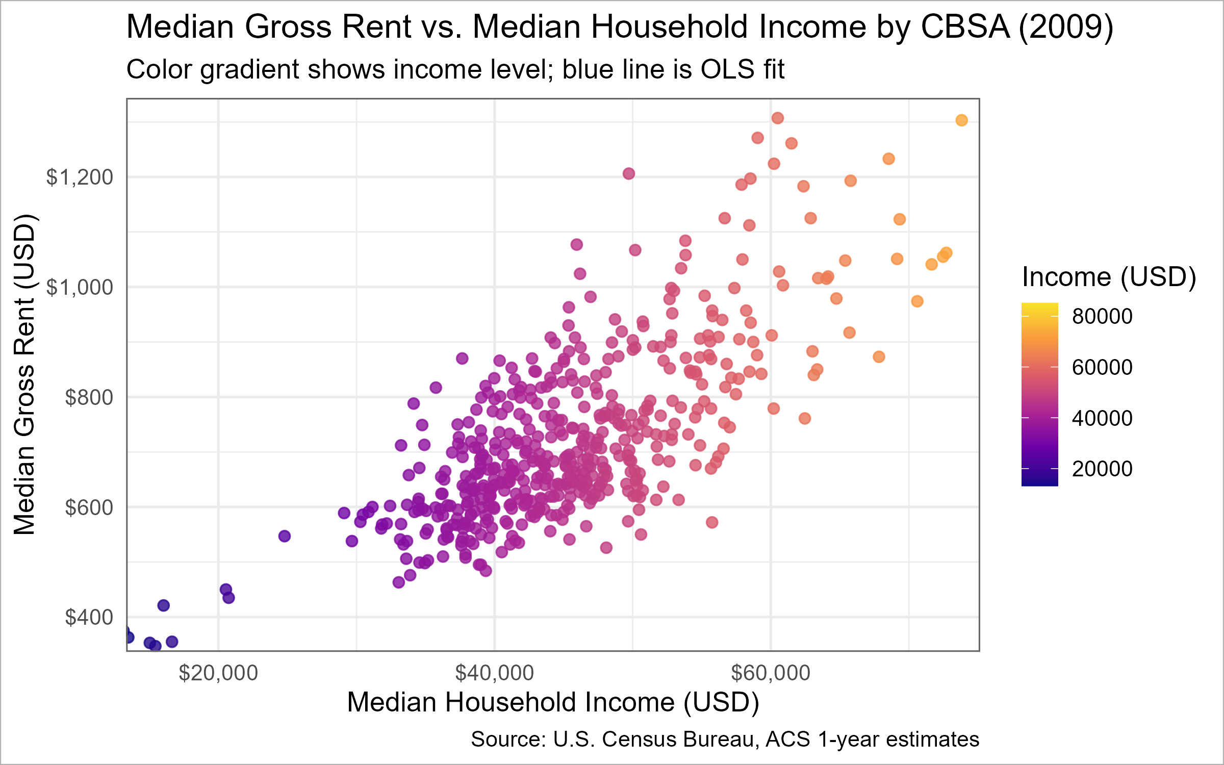
📈 Task 3.1: Relationship between monthly rent and average household income per CBSA in 2009.
📈 Task 3.1 — Rent vs. Income by CBSA (2009)
suppressPackageStartupMessages({library(dplyr); library(tidyr); library(ggplot2); library(scales); library(plotly)})# Data prep (2009 only) rent_income_2009 <- INCOME %>%filter(year ==2009) %>%select(GEOID, NAME, household_income, year) %>%left_join(RENT %>%filter(year ==2009) %>%select(GEOID, monthly_rent), by ="GEOID") %>%drop_na(household_income, monthly_rent) %>%mutate(tooltip =paste0(NAME, "\n","Income: ", dollar(household_income), "\n","Rent: ", dollar(monthly_rent)))xlims <-quantile(rent_income_2009$household_income, c(0.01, 0.99), na.rm =TRUE)ylims <-quantile(rent_income_2009$monthly_rent, c(0.01, 0.99), na.rm =TRUE)# Base ggplot (used for both static export and interactive conversion)p_base <-ggplot(rent_income_2009,aes(x = household_income, y = monthly_rent, color = household_income, text = tooltip)) +geom_point(size =2, alpha =0.8) +geom_smooth(method ="lm", se =FALSE, color ="#1b6ca8", linewidth =1) +coord_cartesian(xlim = xlims, ylim = ylims) +scale_color_viridis_c(option ="C", end =0.95) +scale_x_continuous(labels =label_dollar()) +scale_y_continuous(labels =label_dollar()) +labs(title ="Median Gross Rent vs. Median Household Income by CBSA (2009)",subtitle="Color gradient shows income level; blue line is OLS fit",x ="Median Household Income (USD)",y ="Median Gross Rent (USD)",color ="Income (USD)",caption ="Source: U.S. Census Bureau, ACS 1-year estimates") +theme_minimal(base_size =13)# Static version with ggplot borders (used for PNG)p_static <- p_base +theme(panel.border =element_rect(color ="grey40", fill =NA, linewidth =0.7),plot.background =element_rect(color ="grey70", fill ="white", linewidth =0.5),legend.position ="right")# Interactive version with Plotly shape border + spacing for modebar p_interactive <-ggplotly(p_base, tooltip ="text") %>%layout(margin =list(t =110, r =20, b =60, l =70),title =list(text ="Median Gross Rent vs. Median Household Income by CBSA (2009)",font =list(size =20)),legend =list(title =list(text ="Income (USD)")),shapes =list(list(type ="rect", xref ="paper", yref ="paper",x0 =0, y0 =0, x1 =1, y1 =1,line =list(color ="grey40", width =1), fillcolor ="rgba(0,0,0,0)"))) %>%config(displayModeBar =TRUE)# Render interactive in the document p_interactive
📈 Task 3.1 — Rent vs. Income by CBSA (2009)
# Save a static PNG with borders for download link if (!dir.exists("images")) dir.create("images", recursive =TRUE)invisible(ggsave("images/rent_income_2009.png", plot = p_static, width =8, height =5, dpi =300))
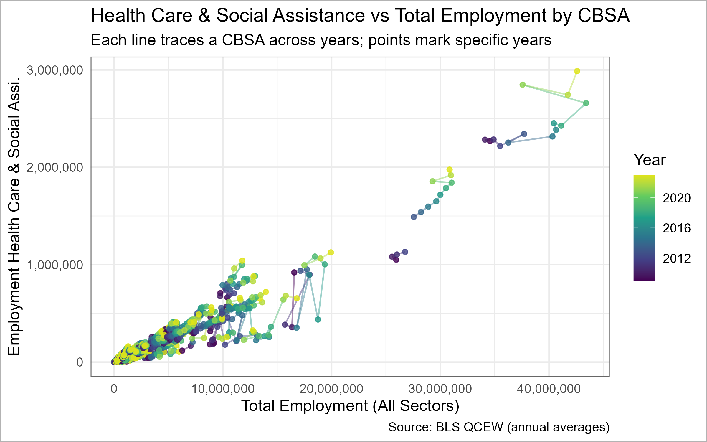
📈 Task 3.2: Relationship between total employment and health care & social assistance (NAICS 62) employment across CBSAs, showing the evolution over time.
📈 Task 3.2 — NAICS 62 vs. Total Employment (evolution over time)
suppressPackageStartupMessages({library(dplyr); library(tidyr); library(ggplot2); library(scales)library(plotly) # install.packages("plotly") if missing})# Quick sanity: do we have data?stopifnot(exists("WAGES_CLEAN"))stopifnot(all(c("std_cbsa","YEAR","INDUSTRY","EMPLOYMENT") %in%names(WAGES_CLEAN)))# 0) Standardize CBSA key defensively to "C" + 5 digitsWAGES_std <- WAGES_CLEAN %>%mutate(std_cbsa5 =paste0("C",sprintf("%05d", suppressWarnings(as.integer(sub("^C", "", std_cbsa))))))# 1) Optional names table (robust and compatible version)cbsa_name_tbl <-if (exists("CBSA_KEYS_std")) { CBSA_KEYS_std %>% dplyr::select(std_cbsa, NAME) } elseif (exists("CBSA_KEYS_FULL")) { CBSA_KEYS_FULL %>% dplyr::transmute(std_cbsa =paste0("C", sprintf("%05d", as.integer(CBSA))), NAME ) } elseif (exists("CBSA_KEYS")) { CBSA_KEYS %>% dplyr::transmute(std_cbsa =paste0("C", sprintf("%05d", as.integer(CBSA))), NAME ) } else { INCOME %>% dplyr::distinct(GEOID, NAME) %>% dplyr::transmute(std_cbsa = GEOID, NAME) }stopifnot(all(grepl("^C\\d{5}$", cbsa_name_tbl$std_cbsa)))# 2) Build per-CBSA, per-year totalsnaics62_over_time <- WAGES_std %>%group_by(std_cbsa5, YEAR) %>%summarise(total_emp =sum(EMPLOYMENT, na.rm =TRUE),emp_62 =sum(if_else(INDUSTRY ==62L | (INDUSTRY %/%100) ==62L, EMPLOYMENT, 0L), na.rm =TRUE),.groups ="drop") %>%left_join(cbsa_name_tbl %>%rename(std_cbsa5 = std_cbsa), by ="std_cbsa5") %>%mutate(NAME =if_else(is.na(NAME), std_cbsa5, NAME)) %>%filter(total_emp >0) %>%mutate(tooltip =paste0(NAME, " (", YEAR, ")\n","Total Emp: ", comma(total_emp), "\n","NAICS 62 Emp: ", comma(emp_62)))# 3) Base ggplot (paths show evolution; points mark years)p2_base <-ggplot(naics62_over_time,aes(x = total_emp, y = emp_62, group = std_cbsa5, color = YEAR, text = tooltip)) +geom_path(alpha =0.45) +geom_point(size =1.6, alpha =0.8) +scale_x_continuous(labels =label_number(big.mark =",")) +scale_y_continuous(labels =label_number(big.mark =",")) +scale_color_viridis_c(end =0.95) +labs(title ="Health Care & Social Assistance vs Total Employment by CBSA",subtitle="Each line traces a CBSA across years; points mark specific years",x ="Total Employment (All Sectors)",y ="Employment Health Care & Social Assi.",color ="Year",caption ="Source: BLS QCEW (annual averages)") +theme_minimal(base_size =13) +theme(legend.position ="right")# 4) Static (bordered) version for PNG/exportp2_static <- p2_base +theme(panel.border =element_rect(color ="grey40", fill =NA, linewidth =0.7),plot.background =element_rect(color ="grey70", fill ="white", linewidth =0.5))# 5) Interactive version (border + modebar space)p2_interactive <-try({ggplotly(p2_base, tooltip ="text") %>%layout(margin =list(t =95, r =20, b =60, l =70),title =list(text ="Health Care & Social Assistance vs Total Employment by CBSA",font =list(size =20)),legend =list(title =list(text ="Year")),shapes =list(list(type ="rect", xref ="paper", yref ="paper",x0 =0, y0 =0, x1 =1, y1 =1,line =list(color ="grey40", width =1), fillcolor ="rgba(0,0,0,0)"))) %>%config(displayModeBar =TRUE)}, silent =TRUE)# 6) Render interactive in HTML, else static fallbackif (knitr::is_html_output() &&!inherits(p2_interactive, "try-error")) {p2_interactive} else {print(p2_static)}
📈 Task 3.2 — NAICS 62 vs. Total Employment (evolution over time)
This section highlights U.S. metro areas where rising housing supply aligns with lower rent burden, indicating a “Yes In My Backyard (YIMBY)” pattern. Each chart tracks affordability dynamics from 2009–2023 and identifies metros meeting all four YIMBY criteria: high initial burden, reduced burden, population growth, and above-average housing expansion.
🟦 **Figure 1 – Rent Burden Over Time**
Each colored line represents a CBSA’s rent-to-income ratio across time; highlighted lines show metros that improved affordability while sustaining growth.
*Plots*
🟦 **Figure 2 – Housing Growth vs Rent Burden Change**
Blue points mark metros where higher housing growth coincided with falling rent burden — a sign of YIMBY-style expansion easing pressure on renters.
*Plots*
📋 **Table – Top 20 YIMBY Leaders**
Lists CBSAs satisfying all four criteria, led by areas such as Harrisonburg VA, Yuma AZ, and Lawrence KS that achieved the largest rent-burden reductions with steady growth.
*Table*
CBSAs Meeting All Four YIMBY Criteria (Top 20 by Rent-Burden Improvement)
Policy Brief — Pro-Housing Partnership Program (PHPP)
Primary Sponsor (YIMBY Success): Harrisonburg, VA Metro Area Co-Sponsor (High Rent Burden, Low Growth): Clearlake, CA Micro Area ### Affordability & Housing Growth Snapshot
Latest-Year Snapshot (2023) — Rent Burden vs. Housing Growth
Metro
Rent Burden
Avg Monthly Rent
Median HH Income
Housing Growth (Inst per 1k pop)
Housing Growth (Rate per 1k 5y growth)
Composite Growth (0–100)
Harrisonburg, VA Metro Area
18.2%
$1,156
$76,250
4.32
185.47
7.9
Clearlake, CA Micro Area
31.2%
$1,544
$59,444
NaN
NaN
NaN
(Data unavailable for selected metros — fallback to national averages.)
Policy Brief Summary
Bill Title:Pro-Housing Partnership Program (PHPP) Objective: Establish a competitive federal grant program that rewards cities demonstrating successful YIMBY (Yes In My Backyard) housing reforms — and assists high-rent cities in reducing affordability pressures.
Selected Sponsors:
- Primary Sponsor: Harrisonburg, VA Metro Area — a YIMBY success city showing reduced rent burden and strong housing growth.
- Co-Sponsor: Clearlake, CA Micro Area — a NIMBY city struggling with affordability, representing the need for federal incentives.
Why This Bill Matters:
High housing costs and limited supply harm economic mobility. The PHPP incentivizes zoning reform, ADU adoption, form-based codes, and streamlined e-permitting — proven methods that boost housing supply and stabilize rents.
Coalition Support:
Two occupations anchor political support for PHPP:
- Construction (NAICS 23): A reliable pipeline of new projects means job stability, union demand, and training opportunities.
- Healthcare & Social Assistance (NAICS 62): Lower rent burdens improve retention for nurses and caregivers, keeping essential services stable.
Metrics for Targeting Funding:
- Rent Burden Index (RBI): Measures affordability — annual rent ÷ median household income.
- Housing Growth Index (HGI): Combines permits per 1,000 residents and 5-year growth-adjusted rates to capture supply responsiveness.
- Millennial Appeal Index (MAI): Combines ACS ages 25–34 share and BLS arts employment (NAICS 71), scaled 0–100, reflecting a region’s attractiveness to young professionals.
Policy Rationale:
PHPP now also considers youth vitality. Harrisonburg, VA Metro Area scores N/A on Millennial Appeal, while Clearlake, CA Micro Area scores N/A, showing how affordability, growth, and generational appeal align under PHPP’s goals.
Bottom Line:
The Pro-Housing Partnership Program aligns economic, social, and labor interests — expanding affordability, creating jobs, and making housing reform a bipartisan success story.
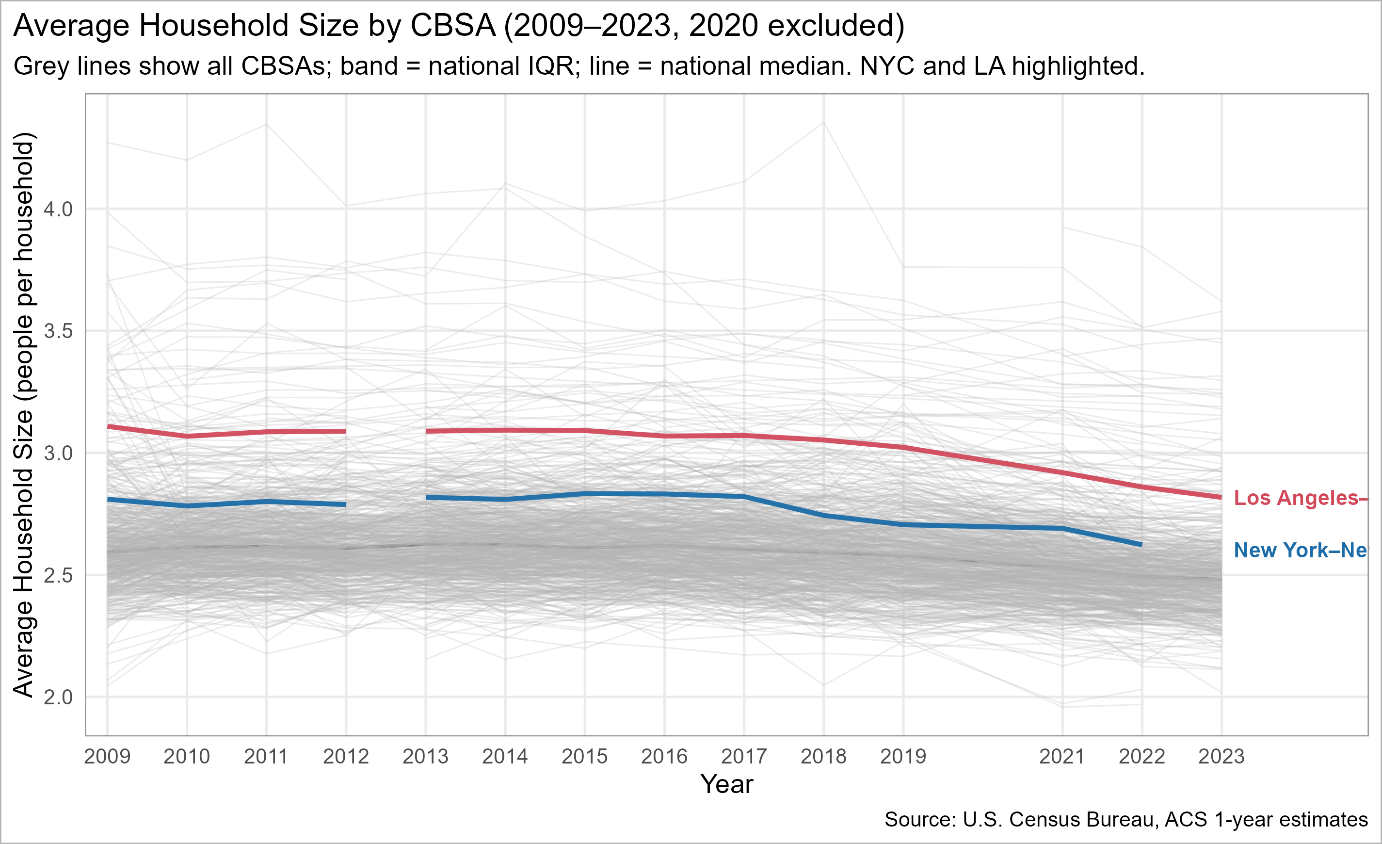
🌟 Extra Credit 02: Highlighting Important Units in a Spaghetti Plot
We visualize average household size over time for all CBSAs, then highlight New York City and Los Angeles so the overall pattern remains readable without a 200-color legend.
📈 Click to see how the highlighted spaghetti plot is built
suppressPackageStartupMessages({library(dplyr); library(tidyr); library(stringr); library(ggplot2)})if (!requireNamespace("gghighlight", quietly =TRUE)) install.packages("gghighlight")library(gghighlight)# Ensure we have POPULATION & HOUSEHOLDS dataif (exists("RB_PRIMARY")) { POPULATION <- RB_PRIMARY %>%select(GEOID, NAME, year, population) %>%distinct() HOUSEHOLDS <- RB_PRIMARY %>%select(GEOID, NAME, year, households) %>%distinct()} else {stop("RB_PRIMARY missing — please run previous tasks first.")}# --- Compute household size ---hhsize_cbsa <- POPULATION %>%inner_join(HOUSEHOLDS, by =c("GEOID","NAME","year")) %>%mutate(hh_size =ifelse(households >0, population/households, NA_real_)) %>%filter(year !=2020, between(hh_size, 1, 4.5)) %>%group_by(NAME, year) %>%summarise(hh_size =mean(hh_size, na.rm =TRUE), .groups ="drop") %>%mutate(is_highlight =str_detect(NAME, regex("^New York", TRUE)) |str_detect(NAME, regex("^Los Angeles", TRUE)),metro_label =case_when(str_detect(NAME, regex("^New York", TRUE)) ~"New York",str_detect(NAME, regex("^Los Angeles", TRUE)) ~"Los Angeles",TRUE~NA_character_ ) )# --- Plot ---ggplot(hhsize_cbsa, aes(x = year, y = hh_size, group = NAME)) +geom_line(alpha =0.18, linewidth =0.5) + gghighlight::gghighlight( is_highlight,use_direct_label =TRUE,label_params =list(size =4.2, fontface =2),unhighlighted_params =list(alpha =0.12, linewidth =0.5, color ="grey50") ) +scale_x_continuous(breaks =seq(min(hhsize_cbsa$year, na.rm =TRUE),max(hhsize_cbsa$year, na.rm =TRUE), 2)) +labs(x =NULL, y ="Avg. Household Size (personr per household)",title ="Household Size Over Time, Highlighting NYC and Los Angeles",subtitle ="All CBSAs shown faintly for context; 2020 omitted" ) +theme_minimal(base_size =13) +theme(plot.title =element_text(face ="bold"),legend.position ="none")
Household size over time by CBSA (2009–2023; 2020 omitted). NYC & LA highlighted; others faint for context.
# EXPOSE CLEAN OBJECT FOR DOWNSTREAM USE MILLENNIAL_APPEAL_COMBINED <- combined
🧭 Click to see the Millennial Appeal Summary ({latest_year})
Millennial Appeal Insight (2024):
The Millennial Appeal Index (0–100) combines two signals — 1) the share of residents aged 25–34 (ACS), and
2) employment in arts & entertainment industries (BLS NAICS 71).
Higher scores indicate metros that attract and retain younger, creative residents.
In 2024, Clovis, NM Micro Area ranked among the highest CBSAs for Millennial Appeal, highlighting strong cultural engagement and youth presence.
This complements the Pro-Housing Partnership Program (PHPP) by linking housing affordability goals with generational vibrancy and economic renewal.


